


AP Calculus Cheat Sheat
Hiérarchie des fichiers
| Téléchargements | ||||||
| Fichiers créés en ligne | (37958) | |||||
| TI-Nspire | (24984) | |||||
| mViewer GX Creator Lua | (19577) | |||||
DownloadTélécharger
Actions
Vote :
ScreenshotAperçu

Informations
Catégorie :Category: mViewer GX Creator Lua TI-Nspire
Auteur Author: qwerty123
Type : Classeur 3.6
Page(s) : 16
Taille Size: 1.09 Mo MB
Mis en ligne Uploaded: 04/05/2015 - 16:56:08
Uploadeur Uploader: qwerty123 (Profil)
Téléchargements Downloads: 1554
Visibilité Visibility: Archive publique
Shortlink : http://ti-pla.net/a209410
Type : Classeur 3.6
Page(s) : 16
Taille Size: 1.09 Mo MB
Mis en ligne Uploaded: 04/05/2015 - 16:56:08
Uploadeur Uploader: qwerty123 (Profil)
Téléchargements Downloads: 1554
Visibilité Visibility: Archive publique
Shortlink : http://ti-pla.net/a209410
Description
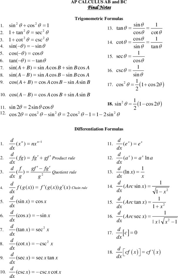
AP CALCULUS AB and BC
Final Notes
Trigonometric Formulas
1. sin θ + cos θ = 1
2 2
sin θ 1
13. tan θ = =
2. 1 + tan 2 θ = sec 2 θ cosθ cot θ
1 + cot 2 θ = csc 2 θ cosθ 1
14. cot θ =
3.
=
4. sin( −θ ) = − sin θ sin θ tan θ
5. cos(−θ ) = cosθ 1
15. secθ =
6. tan(−θ ) = − tan θ cosθ
7. sin( A + B ) = sin A cos B + sin B cos A 16. cscθ =
1
8. sin( A − B ) = sin A cos B − sin B cos A sin θ
cos( A + B ) = cos A cos B − sin A sin B 1
9.
θ
17. cos =
2
(1 + cos 2θ )
2
10. cos( A − B ) = cos A cos B + sin A sin B
1
11. sin 2θ = 2 sin θ cos θ
θ
18. sin =
2
(1 − cos 2θ )
2
12. cos 2θ = cos 2 θ − sin 2 θ = 2 cos 2 θ − 1 = 1 − 2sin 2 θ
Differentiation Formulas
d n d x
1. ( x ) = nx n −1 11. (e ) = e x
dx dx
d d x
2. ( fg ) = fg ′ + gf ′ Product rule 12. (a ) = a x ln a
dx dx
d f gf ′ − fg ′ d 1
3. ( )= Quotient rule 13. (ln x) =
dx g g2 dx x
d d 1
4. f ( g ( x)) = f ′( g ( x)) g ′( x) Chain rule 14. ( Arc sin x) =
dx dx 1− x2
d d 1
5. (sin x) = cos x 15. ( Arc tan x) =
dx dx 1+ x2
d d 1
6. (cos x) = − sin x 16. ( Arc sec x) =
dx dx | x | x2 −1
d
(tan x) = sec 2 x d
7.
dx 17. [c] = 0
dx
d
8. (cot x) = − csc 2 x
dx d
cf ( x ) = cf ' ( x )
dx
18.
d
9. (sec x) = sec x tan x
dx
d
10. (csc x) = − csc x cot x
dx
Integration Formulas
1. ∫ a dx = ax + C
x n +1
∫ x dx = + C , n ≠ −1
n
2.
n +1
1
3. ∫ x dx = ln x + C
∫ e dx = e + C
x x
4.
ax
∫ a dx = +C
x
5.
ln a
6. ∫ ln x dx = x ln x − x + C
7. ∫ sin x dx = − cos x + C
8. ∫ cos x dx = sin x + C
9. ∫ tan x dx = ln sec x + C or − ln cos x + C
10. ∫ cot x dx = ln sin x + C
11. ∫ sec x dx = ln sec x + tan x + C
12. ∫ csc x dx = − ln csc x + cot x + C
∫ sec x d x = tan x + C
2
13.
14. ∫ sec x tan x dx = sec x + C
∫ csc x dx = − cot x + C
2
15.
16. ∫ csc x cot x dx = − csc x + C
∫ tan x dx = tan x − x + C
2
17.
dx 1 x
18. ∫a 2
+x 2
= Arc tan + C
a a
dx x
19. ∫ a2 − x2
= Arc sin + C
a
dx 1 x 1 a
20. ∫x x2 − a2
=
a
Arc sec + C = Arc cos + C
a a x
Formulas and Theorems
1. Limits and Continuity:
A function y = f (x) is continuous at x = a if
i). f(a) exists
ii). lim f ( x ) exists
x→a
iii). lim f ( x ) = f (a )
x→a
Otherwise, f is discontinuous at x = a.
The limit lim f ( x ) exists if and only if both corresponding one-sided limits exist and are equal –
x →a
that is,
lim f ( x ) =
L → lim+ f ( x ) =lim− f ( x )
L=
x →a x →a x →a
2. Even and Odd Functions
1. A function y = f (x) is even if f ( − x) = f ( x) for every x in the function’s domain.
Every even function is symmetric about the y-axis.
2. A function y = f (x) is odd if f ( − x ) = − f ( x ) for every x in the function’s domain.
Every odd function is symmetric about the origin.
3. Periodicity
A function f (x ) is periodic with period p ( p > 0) if f ( x + p ) = f ( x) for every value of x
.
2π
Note: The period of the function y = A sin( Bx + C ) or y = A cos( Bx + C ) is .
B
The amplitude is A . The period of y = tan x is π .
4. Intermediate-Value Theorem
A function y = f (x) that is continuous on a closed interval [a, b] takes on every value
between f ( a ) and f (b) .
Note: If f is continuous on [a, b] and f (a ) and f (b) differ in sign, then the equation
f ( x) = 0 has at least one solution in the open interval (a, b) .
5. Limits of Rational Functions as x → ±∞
f ( x)
i). lim = 0 if the degree of f ( x) < the degree of g ( x)
x →±∞ g ( x )
x2 − 2 x
Example: lim =0
x3 + 3
x →∞
f ( x)
ii). lim is infinite if the degrees of f ( x) > the degree of g ( x)
x → ±∞ g ( x )
x3 + 2 x
Example: lim = ∞
x2 − 8
x →∞
f ( x)
iii). lim is finite if the degree of f ( x) = the degree of g ( x)
x → ±∞ g ( x )
2 x2 − 3x + 2 2
Example: lim = −
10 x − 5 x 2
x →∞ 5
6. Horizontal and Vertical Asymptotes
1. A line y = b is a horizontal asymptote of the graph y = f (x) if either
=
lim f ( x) b=
or lim f ( x) b .(Compare degrees of functions in fraction)
x →∞ x →−∞
2. A line x = a is a vertical asymptote of the graph y = f (x) if either
lim+ f ( x) = ±∞ or lim− f ( x ) = ±∞ (Values that make the denominator 0 but not
x→a x→a
numerator)
7. Average and Instantaneous Rate of Change
i). Average Rate of Change: If ( x0 , y0 ) and ( x1 , y1 ) are points on the graph of
y = f (x) , then the average rate of change of y with respect to x over the interval
[x0 , x1 ] is f ( x1 ) − f ( x0 ) = y1 − y 0 = ∆y .
x1 − x0 x1 − x0 ∆x
ii). Instantaneous Rate of Change: If (x0 , y 0 ) is a point on the graph of y = f (x) , then
the instantaneous rate of change of y with respect to x at x0 is f ′( x0 ) .
8. Definition of Derivative
f ( x + h) − f ( x ) f ( x ) − f (a )
f ′( x) = lim or f ' ( a ) = lim
h →0 h x →a x −a
The latter definition of the derivative is the instantaneous rate of change of f ( x ) with respect to
x at x = a.
Geometrically, the derivative of a function at a point is the slope of the tangent line to the graph of
the function at that point.
9. The Number e as a limit
n
1
i). lim 1 + =
e
n →∞
n
lim (1 + n ) =
1/ n
ii). e
n →0
10. Rolle’s Theorem (this is a weak version of the MVT)
[ ]
If f is continuous on a, b and differentiable on (a, b ) such that
f (a ) = f (b) , then there
is at least one number c in the open interval (a, b ) such that f ′(c) = 0 .
11. Mean Value Theorem
If f is continuous on [a, b] and differentiable on (a, b ) , then there is at least one number c
f (b) − f (a )
in (a, b ) such that = f ′(c) .
b−a
12. Extreme-Value Theorem
If f is continuous on a closed interval [a, b] , then f (x) has both a maximum and minimum
on [a, b] .
13. Absolute Mins and Maxs: To find the maximum and minimum values of a function y = f (x) ,
locate
1. the points where f ′(x) is zero or where f ′(x) fails to exist.
2. the end points, if any, on the domain of f (x) .
3. Plug those values into f (x) to see which gives you the max and which gives you this
min values (the x-value is where that value occurs)
Note: These are the only candidates for the value of x where f (x) may have a maximum or a
minimum.
14. Increasing and Decreasing: Let f be differentiable for a < x < b and continuous for a
a ≤ x ≤ b,
1. If f ′( x) > 0 for every x in (a, b ) , then f is increasing on [a, b] .
2. If f ′( x) < 0 for every x in (a, b ) , then f is decreasing on [a, b ] .
15. Concavity: Suppose that f ′′(x) exists on the interval (a, b )
1. If f ′′( x) > 0 in (a, b ) , then f is concave upward in (a, b ) .
2. If f ′′( x) < 0 in (a, b ) , then f is concave downward in (a, b ) .
To locate the points of inflection of y = f (x) , find the points where f ′′( x ) = 0 or where
f ′′(x) fails to exist. These are the only candidates where f (x) may have a point of inflection.
Then test these points to make sure that f ′′( x) < 0 on one side and f ′′( x) > 0 on the other.
16a. If a function is differentiable at point x = a , it is continuous at that point. The converse is false,
in other words, continuity does not imply differentiability.
16b. Local Linearity and Linear Approximations
The linear approximation to f (x ) near x = x0 is given by y = f ( x0 ) + f ′( x0 )( x − x0 ) for
x sufficiently close to x0 . In other words, find the equation of the tangent line at ( x0 , f ( x0 ) )
and use that equation to approximate the value at the value you need an estimate for.
17. ***Dominance and Comparison of Rates of Change (BC topic only)
Logarithm functions grow slower than any power function ( x n ) .
Among power functions, those with higher powers grow faster than those with lower powers.
All power functions grow slower than any exponential function ( a x , a > 1) .
Among exponential functions, those with larger bases grow faster than those with smaller bases.
We say, that as x → ∞ :
f (x) g(x)
1. f ( x ) grows faster than g ( x ) if lim = ∞ or if lim = 0.
x →∞ g(x) x →∞ f (x)
If f ( x ) grows faster than g ( x ) as x → ∞ , then g ( x ) grows slower than f ( x ) as
x→∞.
f (x)
2. f ( x ) and g ( x ) grow at the same rate as x → ∞ if lim = L ≠ 0 (L is finite
x →∞ g(x)
and nonzero).
For example,
ex
1. e x grows faster than x 3 as x → ∞ since lim = ∞
x →∞ x 3
x4
2. x 4 grows faster than ln x as x → ∞ since lim = ∞
x →∞ ln x
x 2 + 2x
3. x 2 + 2x grows at the same rate as x 2 as x → ∞ since lim =1
x →∞ x2
To find some of these limits as x → ∞ , you may use the graphing calculator. Make sure that an
appropriate viewing window is used.
18. ***L’Hôpital’s Rule (BC topic, but useful for AB)
f ( x) 0 ∞ f ′( x)
If lim is of the form or , and if lim exists, then
x→a g ( x) 0 ∞ x → a g ′( x )
f ( x) f ′( x)
lim = lim .
x→a g ( x) x → a g ′( x )
19. Inverse function
1. If f and g are two functions such that f ( g ( x)) = x for every x in the domain of
g and g ( f ( x)) = x for every x in the domain of f , then f and g are inverse
functions of each other.
2. A function f has an inverse if and only if no horizontal line intersects its graph more
than once.
3. If f is strictly either increasing or decreasing in an interval, then f has an inverse.
4. If f is differentiable at every point on an interval I , and f ′( x) ≠ 0 on I , then
−1
g= f ( x) is differentiable at every point of the interior of the interval f (I ) and if
the point ( a, b ) is on f ( x ) , then the point ( b, a ) is on g= f −1
( x) ; furthermore
1
g '(b) = .
f '(a)
20. Properties of y = e
x
1.
x
The exponential function y = e is the inverse function of y = ln x .
2. The domain is the set of all real numbers, − ∞ < x < ∞ .
3. The range is the set of all positive numbers, y > 0 .
4.
d x
dx
(e ) = e x and
d f ( x)
dx
e ( )
= f ' ( x ) e f ( x)
x x x + x2
5. e 1 ⋅e 2 = e 1
6. y = e x is continuous, increasing, and concave up for all x .
7. lim e x = +∞ and lim e x = 0 .
x →∞ x →−∞
8. e ln x = x , for x > 0; ln(e x ) = x for all x .
21. Properties of y = ln x
1. The domain of y = ln x is the set of all positive numbers, x > 0.
2. The range of y = ln x is the set of all real numbers, − ∞ < y < ∞ .
3. y = ln x is continuous and increasing everywhere on its domain.
4. ln (ab ) = ln a + ln b .
a
5. ln = ln a − ln b .
b
6. ln a r = r ln a .
7. y = ln x < 0 if 0 < x < 1 .
8. lim ln x = +∞ and lim ln x = −∞ .
x → +∞ x → 0+
ln x
9. log a x =
ln a
f '( x)
10.
d
dx
( ln f ( x ) ) =
f ( x)
and
d
dx
( ln ( x ) ) =